Wecome to the CeLaVi tutorial

CeLaVi (after Cell Lineage Visualisation tool), is a web-server based visualisation tool that allows any user to interrogate interactively the cell lineage of an organism or population of cells whilst visualising its spatial context and identity of the cells.
CeLaVi is built using HTML5, Ajax, jQuery, CSS and the visualisation libraries D3.js and Plotly.js. It does not need to be installed and has been tested on the following browsers and OS:

OS	Version	Chrome	Firefox	Safari
Linux	Ubuntu 16.04	87.0.4280	83.0	n/a
MacOS	10.15.2	87.0.4280	83.0	13.1.2
Windows	10	87.0.4280	83.0	n/a

1. Input files

To visualize a Cell Lineage Tree and relate it to a 3D cell map, the user needs to provide two files: 1) Cell lineage tree file and 2) 3D coordinates file. Below we explain how to upload these files and what is the specific format for each.

1.1 Cell lineage tree file

The tree file needs to be uploaded either in Newick or Json format. To upload a tree file, click the "Upload tree (select format)" box and choose the file to upload. If the selected file has a correct extension, i.e. “.nw” or “.newick” for newick or “.json” for json files, the tree will automatically be shown.

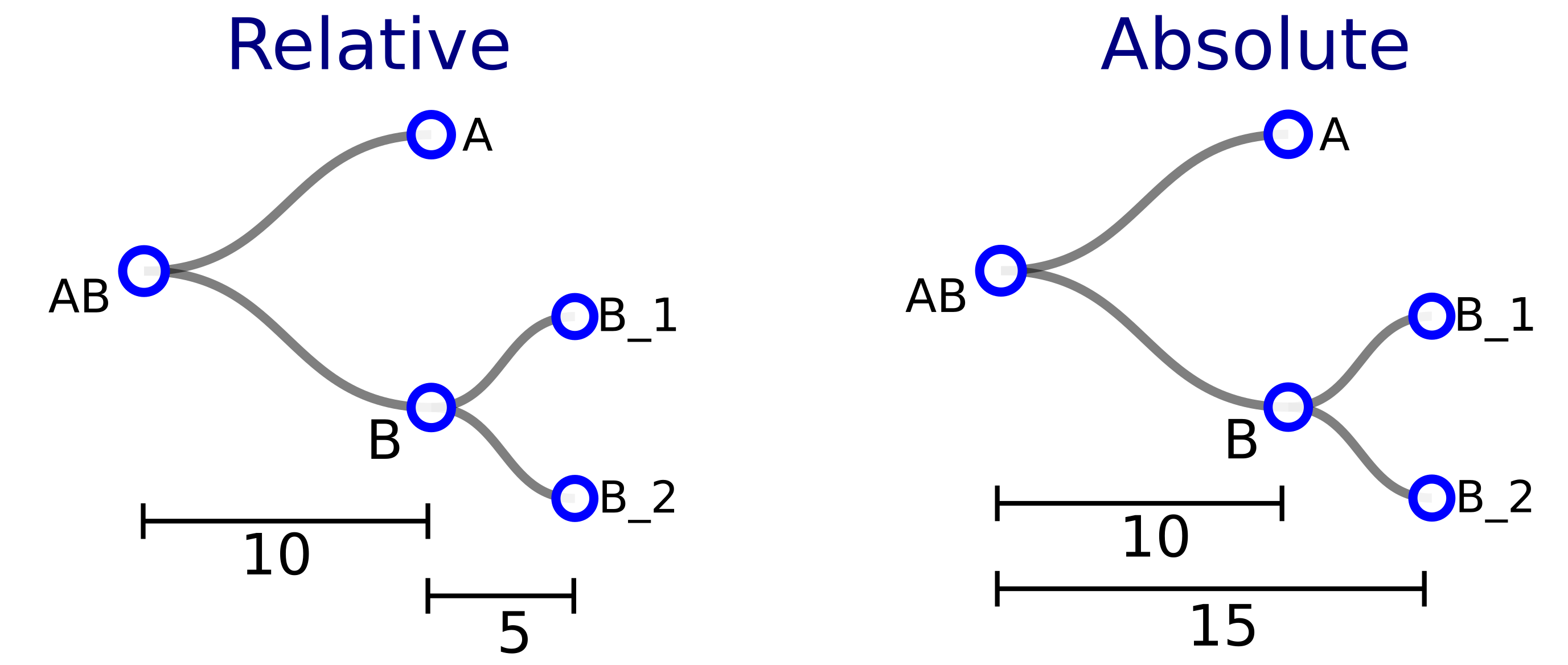
1.1.1 About branch-lenght modes

For lineage tree files containing branch length information (timing of cell divisions) a dialog box will appear allowing the user to specify how branch lengths should be plotted: if branch lengths represent time to the parent node the user should write "relative" in the dialog box and then click on “OK”. If they represent time from the root, then the user needs to write "absolute" and then click “OK”. If the user clicks on “Cancel” instead, branch lengths will be ignored. For more details on the structure of the input files please download the Test Files.
Below we show in a schematic diagram how the same tree would be encoded in a json file usign either the "relative" or "absolute" mode. After selecting the approapriate mode, the tree depicted is the same.

1.2 3D coordinates file

The file containing the 3D coordinates of the cells must contain a table in comma- separated-value (csv) format. The first line is a header or descriptor line, which specifies the column’s identity as “cell”, “X”, “Y”, and “Z”. Each subsequent line corresponds to one cell. The first column contains the cell ID, and the next columns are the three coordinate values (X,Y and Z, respectively).

1.3 Store and display the data source

There is an option to store the data source metadata in both the lineage tree and 3D coordinates files. If a file contains this metadata, the source information will be displayed at the bottom of the corresponding viewer, like in the example datasets. Below we describe how to add the data source to the files.

JSON file

In the field corresponding to the descriptor of the first cell, add

{"species”:“xxx”, “source”:”yyy”,

where “xxx” is the name of the species, and “yyy” the source information to display. Take care of including a comma after the source name, as indicated in the example below:

{"species":"NA (In silico organoid)","source":"Germann et al (2019). doi:10.1016/J.CELS.2019.02.007",

NEWICK file

Introduce the following 2 lines at the top of the file:

[Species:xxx];
[Source:yyy];

where "xxx" is the name of the species, and "yyy" the source information to display, just as in the following example:

[Species: Ciona intestinalis];
[Source: Manually created based on Conklin nomenclature (Conklin EG, 1905)];

CSV 3D coordinates file

In the header line, after the last coordinate column in the header (typically Z), add the following text after the comma:

[Source: xxxxx]

Where "xxx" is the text describing the source, as in the example header below:

clone,cell,X,Y,Z,[Source: Germann et al (2019). doi:10.1016/J.CELS.2019.02.007]

Open input files

2. Interacting with the Lineage tree

By default, any cell in the tree is labeled either in blue or white, representing one of two states: a "collapsed" state (labeled in blue), in which its daughter cells are hidden, or an "expanded" state (labeled in white), in which its daughter cells are shown. Terminal cells in the tree do not have daughters, and are by definition in the "expanded" state. When a cell lineage tree is uploaded, by default the tree is shown as completely expanded.

2.1 Collapsing/Expanding the daughters of one cell

In order to switch between the "collapsed" (blue) and "expanded" (white) states of an internal node, right-click on the node and select “Collapse node [node ID]”/ “Expand node [node ID]”. This will expand just the daughters of the node in question.

2.2 Collapsing/Expanding all descendants of one cell

To collapse or expand all the descendants of a node (daughters, granddaughters etc.), right-click on the node and select “Collapse all until here”/ “Expand all from here”.

2.3 Collapsing/Expanding all cells from a given tree depth

This is an option to expand/collapse daughters of many cells at once by using the "Tree depth" section below the cell lineage. When loading a tree, CeLaVi displays the different depths of the tree as purple circles in the "Tree depth" section. These circles, as well as showing the number of depth levels, can be used to collapse/expand all the cells at a given tree depth: click the depth level of interest, select the option "Collapse all cells" or "Expand all cells".
Please note that the tree levels are defined in ascending order, starting with the root at level 0, the daughters of the root as level 1, and so on.

2.4 Delete nodes (prune tree)

It is possible to delete nodes in the Lineage tree, which can be useful when dealing with lineage trees with thousands of cells or when the user wants to focus on a specific clone. If the user wants to delete a specific node, it can be done by right clicking on that node and select the option “Delete this node” from the menu.
There is also the option to delete multiple nodes, from a given tree depth, that have fewer descendants than a desired threshold. For this, click on the desired tree depth (in the Tree depth section at the bottom of the lineage viewer) and select the option “Delete nodes with fewer than N descendants”. This will prompt an input box where the user needs to enter an integer number and to click “OK” for confirmation. The entered number will specify the number of descendants to be used as a threshold.
Importantly, the pruning of the tree does not affect the original input file, so the user can restart by loading again the lineage file.

2.5 Collapse extra cells

It is possible that, when loading a dataset, the user finds there are more terminal cells in the Lineage tree than cells in the 3D viewer, producing a mismatch between both visualisations. To account for this, the user can collapse all the cells that are not found in the 3D viewer by clicking on “Collapse extra cells” in the “Other options” dropdown menu. This function collapses all internal nodes whose terminal leaves are not found in the 3D viewer area. Terminal cells in the lineage tree that are not found and cannot be collapsed are painted gray.

2.6 Delete extra cells

If the user wants to delete the extra cells from the tree completely (and not just collapsing them like above) the “Delete extra cells option” can be used. This function deletes all the both the internal nodes whose terminal cells are not found in the 3D viewer area and terminal cells that cannot be found in the 3D viewer. The pruning of the tree does not affect the original input file, so the user can restart by loading again the lineage file.

2.7 Reset view

The button “Reset view” at the bottom of the Lineage viewer resets the Lineage tree to the initial visualisation, i.e. all nodes expanded and with the tree centered in the lineage viewer). This function does not recover the deleted nodes on the tree. If some nodes have been deleted from the tree by the user, the lineage tree needs to be loaded again (selecting it again as input file) to recover the deleted nodes.

2.8 How to deal with very large datastets

Rendering a lineage tree with thousands of cells can be computationally intensive on the client side (user’s computer). Although the maximum number of cells and cell lineage nodes that can be visualised without experiencing delays would depend on the client computer, we have noted that CeLaVi typically becomes less responsive when more than 10,000 cells are loaded.
In order to reduce the computational burden of dealing with such trees, CeLaVi has an option to plot only some of the branches of the tree, which is automatically selected when the number of cells is greater than 500. This function is only relevant, however, when the lineage tree is not completely resolved, i.e. some internal nodes have more than 2 daughters (polytomies). This is a common case in clonal analyses, where cells are grouped in clones but the inter-clonal relationships are not resolved. When the “Render only some branches” is selected, only the first and last branches are plotted in each polytomy, potentially reducing massively the amount of lines that need to be plotted (see video of this function with the organoid example). This option can be changed by the user by clicking on “Render all branches”.
Another way of increasing the respo esponsiveness of the Lineage viewer is to reduce the number of elements displayed in the Lineage viewer, for example by showing only the root node label (click on the “0” Tree depth level and selecting “Show label until this depth”) or by collapsing non-relevant nodes in the tree. Also, if the user is interested in a specific clone, it is possible to export the clone as a JSON file (see “Exporting a clone to a JSON file” section). This file can be loaded and visualised subsequently in CeLaVi, with the original coordinates and annotation files.

Collapse/Expand tree

Tree depth

Delete extra cells

Render all/some branches

3. Interacting with cells in the 3D viewer

The 3D visualisation is implemented using the 3D scatterplot function of plotly.js, a visualisation library based on d3.js and stack.gl For more information on the plotly.js visualisation library visit https://plot.ly/javascript/.

3.1 Rotate/zoom/pan

When a file of 3D cell locations has been uploaded, the positions of all cells are shown in the 3D viewer on the right hand side of the screen. It is possible to Zoom in/out by using the scroll wheel of the mouse, to rotate by left-clicking and dragging, and to pan the 3D scatterplot by right-clicking and dragging the mouse.

3.2 Modifying the representation of cells

The user can modify some features of the 3D viewer area using the "3D cell controls" panel, located in the bottom right of the 3D viewer area.
On the left, the "Reset colors" button resets the colour of the cells in both the lineage and 3D viewer to the default (light grey). The “Reset clones” button deletes the saved list of clones. The size of the cells can be modified using the “Cell size” input box either by changing the size of the cells in a stepwise manner using the arrow buttons or by typing an integer value.
There are also 2 checkboxes in this section: 1) The “Show Axes” checkbox allows the user to show or hide the 3D axes plotted in the background. 2) The “Show lineage” option allows the user to visualise the degree of lineage relationship for each of the cells relative to a selected cell. Every cell is coloured using a heatmap that shows how closely related each cell is to the selected cell. To do this, select the “show lineage” option by clicking on the checkbox and then click on any cell in the 3D viewer area.

3.3 Highlighting the lineage history of a cell

An important feature of CeLaVi is the possibility of interactively interrogating the data. One useful function is to highlight the developmental lineage of any cell chosen in the 3D visualisation area. Clicking on any cell in the 3D visualisation will change its colour to red and its lineage will be highlighted in red on the lineage tree. More specifically, the cell that has been clicked will be coloured in red as will all its ancestors down to the root. Note: To do this, the lineage tree (or at least the clade of the cell to be highlighted) needs to be completely expanded.
Note: To do this, the lineage tree (or at least the clade of the cell to be highlighted) needs to be completely expanded.

3.4 Hide 3D cells missing in Lineage tree

In the case a 3D cells file is loaded and it contains more cells than found in the Lineage tree, a warning message will be shown specifying the number of cells that were not found in the tree. The “missing” cells will be plotted on the 3D viewer but without a fill colour, making them easily identifiable. The user can then hide/show these cells on the 3D viewer by clicking on the “Cells missing in tree” legend at the top right of the 3D viewer (see video).

Interacting with cells in the 3D viewer

4. Visualising clones

4.1 Showing a single clone

There are two ways to visualise the spatial distribution of all the descendants of a given cell in the cell lineage. The first is simply by clicking on any cell in the Lineage tree. This will mark all the descendant cells on the 3D visualisation section by assigning them a random colour. With this option we can mark multiple clones at the same time.
Another option is to hover the cursor over any cell in the lineage tree. In this case, all cells that do not belong to the selected clone will be faded out in the 3D viewer whilst the mouse cursor is on the ancestral cell of interest. This function only allows visualisation of one clone at a time.
The accompanying video shows both options for highlighting a single clone in the 3D cell section and how to interact with the 3D plot.

4.2 Showing clones from a given tree depth

It is possible to mark all the clones at a given tree depth by interacting with the "Tree depth" section below the Lineage Tree. In the accompanying video this function is shown using the Parhyale dataset. Clicking on the depth level 1 circle we can then select the option "Show clones from this depth". This marks the spatial distribution of the 20 clones that comprise this dataset. We can also use this option to see how a clone gets divided into subclones in the subsequent cell divisions. For this we need to expand only the clone(s) we are interested in following, and then select the option "Show clones from this depth" for increasing depths.

4.3 Showing clones arising at a given time point

When the Cell Lineage file contains branch length information (which essentially represents the timing of cell divisions), it is also possible to show all the clones originating at a given time point. To do this, first click the box "Branch Len" to change the representation of the Lineage tree so that it shows branch lengths. The "Tree depth" section at the bottom of the Lineage Tree will change from showing the tree depths (purple circles) to showing an horizontal slider. The horizontal slider represents developmental time (from 0 to 100%) and can be clicked to show the clones originating at different time points. A vertical dashed line is plotted on top of the Lineage Tree showing the selected level. It is also possible to expand only those clones in the lineage tree that the user wants to visualise. The following video shows how to visualise clones at a given tree depth or at a given time point.

4.4 Saving clones

If the user is interested in one or several specific clones, it is possible to save these as a list that can be used to visualise them later. In the Lineage tree we right-click on the tree node (parent cell) of interest and select the option "Save clone [cell ID]". A colour picker will be displayed allowing the user to choose the colour of the cells of this clone when selected. After choosing the colour and clicking “OK” in the colour picker box, the ID of the cell will be saved into a list that can be displayed by clicking on the button "Saved clones". We can recall a saved clone by clicking on its identity in this list. The cells of the selected clone will then be highlighted by its chosen colour. It is possible to delete the saved list of clones by clicking on the “Reset Clones” button.

4.5 Export clones as a cell annotations file

It is possible to export the saved list of clones as a csv file. This csv file can be loaded as a “cell annotations file” to visualise the clones in another CeLaVi session, or to share the clones' list with other people.
For more information on cell annotations file see the section below. The video shows how to save clones, how to select them from the list to display them and how to export them as a cell annotations file.

4.6 Exporting a clone to a JSON file

With this function, it is possible to export the complete lineage information of any selected clone (all tree levels, not only the final time point), together with the cell IDs and branch lengths of all the descendants, as a JSON file in the user's computer.
This file can be loaded and visualised subsequently in CeLaVi, with the original coordinates and annotation files. This feature is useful for users that want to focus on, or easily share, a specific clone. The accompanying video shows the exporting of the EMS lineage in C. elegans. Note that when loading a 3D coordinates file again, the cells that are missing are shown only with a blue outline. The user can hide these cells by clicking on the box "Cells missing in tree" on the right top of the 3D viewer".

Showing a single clone

Showing various clones

Saving clones

Exporting clones as JSON

5. Cell annotations

Apart from the cell lineage and spatial distribution of the cells, it is possible to visualise additional information, e.g. cell type.

5.1 Uploading a cell annotation file

To upload a file, click on the “Cell annotations file” input box and select the file from your computer. The file needs to be a csv file with 2 columns. The first column should have the cell ID (which must be identical to its entry in the 3D coordinates file), and the second column will show the cell annotation the user wants to visualise, as cell type (e.g. neuron). If the file format is correct, a table will display containing all cell type annotations as coloured rows.

5.2 Visualising cell annotations

The cell annotations table serves for interactively visualising the different sets of annotated cells in the 3D viewer and the lineage tree. The video shows how it works with the Ciona gastrula dataset example. Here, the cell annotations correspond to the different cell types (or fates) in the gastrula. When hovering over a table row, the cells that belong to that cell type are highlighted by fading out the rest of the cells. If the row is clicked, the cells in both the 3D viewer and the lineage viewer are painted with the colour matching the background colour of the row that has been clicked.

Cell annotations

6. Visualising gene expression

An additional feature of CeLaVi is the possibility of visualising gene expression information. Such information can have been generated by different technologies, like single cell sequencing or in situ sequencing.

6.1 Uploading a gene expression file

The gene expression file needs to be a csv file with genes as rows and cells as columns and it needs to contain a header with the format “gene,cell_01,cell_02,cell_03”.
As with the cell annotations file, the cell ID must be identical to the cell IDs used in both the 3D cells and lineage tree files.

6.2 Plotting gene expression

After successful loading of the gene expression file, a gene search box will appear above the 3D viewer. To plot the expression of a gene of interest, type its name in the search box and click on the “submit” button. The search box has an autofill function, so a list of genes starting with the letter(s) initially entered will display when typing the name of a gene of interest. The gene expression values will be represented on the 3D and lineage viewers using a heatmap. The heatmap scale (level of expression) will be plotted at the bottom of the 3D viewer area. The accompanying video shows how to upload and visualise gene expression data using the Ciona gastrula example dataset.

6.3 Plotting other quantitative variables

The gene expression highlighting option can be used to plot any other quantitative feature associated with the cells (UMI, mitochondrial gene expression, etc). For this, the user just needs to upload a file with the same format as a the gene expression file. The quantitative information file needs to be a csv file with the features to display as rows and cells as columns, and it needs to contain a header with the format “gene,cell_01,cell_02,cell_03” with the cell ID identical to the cell IDs used in both the 3D cells and lineage tree files.
After successful loading of the custom quantitative data file, use the gene search box that will appear above the 3D viewer. To plot the quantitative feature of interest, type its name in the gene search box and click on the “submit” button. The quantitative information (i.e. UMIs) will be represented on the 3D and lineage viewers using a heatmap. The heatmap scale (level of expression) will be plotted at the bottom of the 3D viewer area.

Gene expression

7. Exporting visualisations as images

7.1 Exporting the Lineage tree as an image

At any point, the lineage tree displayed in the lineage viewer can be exported as an image in SVG or PNG format. To do this, select the desired image format from the dropdown menu shown when hovering on the button “Save Image” at the bottom of the lineage viewer.

7.2 Exporting 3D cells as an image

As with the lineage tree, the 3D cells can be exported at any time as a PNG image. To do this, select the PNG option from the dropdown menu shown when hovering over the button “Save Image” at the bottom of the 3D viewer.

8. About test files

8.1 Caenorhabditis elegans

The embryonic cell lineage of the nematode C. elegans was described by John Sulston and collaborators in 1983[1]. The data used for the cell lineage and the cell types were extracted from a json file available made available by Nikhil Bhatla at wormweb.org/celllineage
The 3D coordinates come from the study of Fuhui Long and collaborators[2], where they mapped 357 cells (out of the 558 cells) of the L1 larval stage, using confocal image stacks of 15 individual worms.

8.2 Ciona gastrula

The cell lineage of the ascidian Ciona intestinalis was described by Edward Conklin in 1905[3]. The cell lineage file (in newick format) was created using Conklin's nomenclature, from the zygote to the 110-cells stage.
The 3D coordinates of the Ciona gastrula were obtained from a reconstructed 3D embryo model[4] available in the Aniseed database[5].The 3D embryo model contains, for each cell, a set of data points in space (point cloud) representing the shape in 3D. To represent each cell as a single point in the 3D space we used the calculated centroid of the point cloud of each cell.
The gene expression dataset was obtained from the single cell sequencing dataset by Michael Levine and collaborators[6]. We used the "expression_matrix_C110.1.tsv" raw expression data matrix (expression levels of 15,307 genes in 1,731 cells) together with the metadata associated file.
"C110.1.clusters.upload.rename.1.txt" that contains the cell type identity of each cell at the early gastrula stage. We used the R software version 3.6.3[7] with the Seurat package version 3.1.4[8] to calculate the 500 most variable genes and to obtain their average expression values per cell. The gene names correspond to human gene IDs, derived from the Ciona intestinalis genome assembly KH2012 with NCBI Gene Model to Best Blast Hit mapping, available in the Aniseed database. Only the gene ID with the highest Blast e-value is shown.

8.3 Parhyale limb

The cell lineage and 3D coordinates of the limb of the crustaean Parhyale hawaiensis were obtained by Tassos Pavlopoulos and collaborators[9]. They imaged transgenic fluorescently-labeled embryos with multi-view light-sheet microscopy at high spatiotemporal resolution over several days of embryogenesis. The cell lineage was then reconstructed with the aid of the MaMuT software.

8.4 In silico Organoid

The "organoid" dataset comes from a simulation of morphogenesis using the ya||a software[10]. The organoid is the product of a branching morphogenesis simulation with epithelium and mesenchyme (only the epithelium is used for the example). The simulation was kindly provided by Miquel Marín-Riera, coauthor of the ya||a software, and is based on the example "branching.cu" available in https://github.com/germannp/yalla.